
1. IMDB 영화평을 이용한 지도학습 기반 감성분석
- https://www.kaggle.com/c/word2vec-nlp-tutorial/data
- 데이터 구조
- id : 유저 아이디
- sentiment : 감성. 긍정 1, 부정 0
- review : 리뷰
- 레이블이 있는 데이터를 가지고 범주를 예측하는 것과 동일하지만, 자연어는 피처가 문장으로 주어지기 때문에 문장을 피처 벡터화 작업해줘야 하는 것이 다르다.
- 모든 단어를 각각의 피처로 만들고 각 문장은 피처의 존재 여부를 데이터로 소유한다.
1. 데이터 읽어오기
import pandas as pd

review_df = pd.read_csv('./data/IMDB/labeledTrainData.tsv/labeledTrainData.tsv', header=0, sep="\t", quoting=3)
review_df.head(3)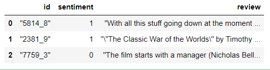 |
2. 데이터 전처리
- <br />를 제거: replace
- 영문만 남겨두기: 정규식 모듈의 sub 메소드 활용
#정규식 모듈
import re

# <br> html 태그 -> 공백으로 변환
review_df['review'] = review_df['review'].str.replace('<br />',' ')

# 파이썬의 정규 표현식 모듈인 re를 이용하여 영어 문자열이 아닌 문자는 모두 공백으로 변환
review_df['review'] = review_df['review'].apply( lambda x : re.sub("[^a-zA-Z]", " ", x) )

print(review_df['review'].head())| 0 With all this stuff going down at the moment ... 1 The Classic War of the Worlds by Timothy ... 2 The film starts with a manager Nicholas Bell... 3 It must be assumed that those who praised thi... 4 Superbly trashy and wondrously unpretentious ... Name: review, dtype: object |
- a-zA-Z가 아닌 글자를 공백으로 치환
- 한글을 제외한 글자 제거: [^가-힣]
3. 훈련/테스트 데이터 분리
- 지도학습 기반의 분류이므로 훈련 데이터를 이용해서 훈련하고, 테스트 데이터로 확인하는 것을 권장
from sklearn.model_selection import train_test_split

class_df = review_df['sentiment']
feature_df = review_df.drop(['id','sentiment'], axis=1, inplace=False)

X_train, X_test, y_train, y_test= train_test_split(feature_df, class_df, test_size=0.3, random_state=156)

X_train.shape, X_test.shape| ((17500, 1), (7500, 1)) |
4. 피처벡터화
- CountVectorizer로 피처벡터화 수행 후 분류 모델 훈련
- TdidfVectorizer로 비처벡터화 수행 후 분류 모델 훈련
from sklearn.feature_extraction.text import CountVectorizer, TfidfVectorizer
from sklearn.pipeline import Pipeline
from sklearn.linear_model import LogisticRegression
from sklearn.metrics import accuracy_score, roc_auc_score
# 스톱 워드는 English, filtering, ngram은 (1,2)로 설정해 CountVectorization수행.
# LogisticRegression의 C는 10으로 설정.
pipeline = Pipeline([
('cnt_vect', CountVectorizer(stop_words='english', ngram_range=(1,2) )),
('lr_clf', LogisticRegression(C=10))])
# Pipeline 객체를 이용하여 fit(), predict()로 학습/예측 수행. predict_proba()는 roc_auc때문에 수행.
pipeline.fit(X_train['review'], y_train)
pred = pipeline.predict(X_test['review'])
pred_probs = pipeline.predict_proba(X_test['review'])[:,1]
print('예측 정확도는 {0:.4f}, ROC-AUC는 {1:.4f}'.format(accuracy_score(y_test, pred),
roc_auc_score(y_test, pred_probs)))| 예측 정확도는 0.8860 , ROC-AUC는 0.9503 |
# 스톱 워드는 english, filtering, ngram은 (1,2)로 설정해 TF-IDF 벡터화 수행.
# LogisticRegression의 C는 10으로 설정.
pipeline = Pipeline([
    ('tfidf_vect', TfidfVectorizer(stop_words='english', ngram_range=(1,2) )),
    ('lr_clf', LogisticRegression(C=10))])

pipeline.fit(X_train['review'], y_train)
pred = pipeline.predict(X_test['review'])
pred_probs = pipeline.predict_proba(X_test['review'])[:,1]

print('예측 정확도는 {0:.4f}, ROC-AUC는 {1:.4f}'.format(accuracy_score(y_test ,pred),
roc_auc_score(y_test, pred_probs)))| 예측 정확도는 0.8939, ROC-AUC는 0.9596 |
ngram을 설정하면 하나의 단어를 하나로 인식하지 않고, n개의 단어까지 하나의 단어로 인지한다.
영어는 2나 3을 설정: 사람 이름 등 (I am a boy -> I am, am a, a boy)
정확하게 일치하는 것이라면 예측도 가능하다. (I am 다음은 a/an 이구나)
그래서 생성형 AI는 ngram을 설정하는게 좋다.
2. 비지도학습 기반 감성분석
- 레이블이 없는 경우 사용
- Lexicon이라는 감성 분석에 관련된 어휘집을 이용하는 방식
- 한글 버전의 Lexicon이 현재는 제공되지 않음
3. 네이버 식당 리뷰 데이터를 이용한 감성분석
- 이진분류는 LogisticRegression이면 충분
- 크롤링한 데이터
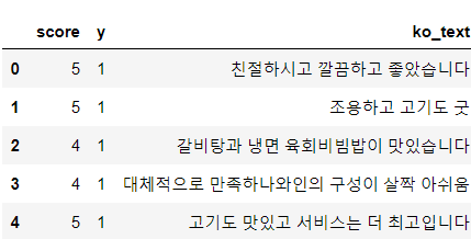
- score: 별점
- y: 감성, score가 4이상이면 1, 아니면 0
1. 데이터 읽어오기
df = pd.read_csv("./python_machine_learning-main/data/review_data.csv")
print(df.head())| score review y 0 5 친절하시고 깔끔하고 좋았습니다 1 1 5 조용하고 고기도 굿 1 2 4 갈비탕과 냉면, 육회비빔밥이 맛있습니다. 1 3 4 대체적으로 만족하나\n와인의 구성이 살짝 아쉬움 1 4 5 고기도 맛있고 서비스는 더 최고입니다~ 1 |
2. 데이터 전처리
한글 추출: (가-힣)
- 모음과 자음만으로 구성된 텍스트도 추출하려면 (ㄱ-ㅣ, 가-힣)
#한글을 제외한 글자 전부 제거
import re
# 텍스트 정제 함수 : 한글 이외의 문자는 전부 제거
def text_cleaning(text):
    # 한글의 정규표현식으로 한글만 추출합니다.
    hangul = re.compile('[^ ㄱ-ㅣ가-힣]+')
    result = hangul.sub('', text)
    return result
df['ko_text'] = df['review'].apply(lambda x: text_cleaning(x))
del df['review']
df.head()- 데이터 용량을 줄이기 위해 바로바로 del
 |
3. 형태소분석
from konlpy.tag import Okt

# konlpy라이브러리로 텍스트 데이터에서 형태소를 '단어/품사'로 추출
def get_pos(x):
    tagger = Okt()
    pos = tagger.pos(x) # PartOfSpeech
    pos = ['{}/{}'.format(word,tag) for word, tag in pos]
    return pos
# 형태소 추출 동작을 테스트합니다.
result = get_pos(df['ko_text'][0])
print(result)| ['친절하시고/Adjective', '깔끔하고/Adjective', '좋았습니다/Adjective'] |
4. 피처 벡터화
- 등장하는 모든 단어를 수치화
# 등장 횟수만을 고려한 피처 벡터화를 위한 사전 생성하고 데이터를 피처 벡터화
from sklearn.feature_extraction.text import CountVectorizer

# 형태소를 벡터 형태의 학습 데이터셋(X 데이터)으로 변환
index_vectorizer = CountVectorizer(tokenizer = lambda x: get_pos(x))
X = index_vectorizer.fit_transform(df['ko_text'].tolist())

X.shape| (545, 3030) |
- 3030: 단어의 개수
- 545: 행의 개수
print(df['ko_text'][0])
print(X[0])| 친절하시고 깔끔하고 좋았습니다 (0, 2647) 1 (0, 428) 1 (0, 2403) 1 |
- 다 한번씩만 등장!
#CounterVectorizer를 이용해서 만든 피처 벡터를 Tfidf 기반으로 변경
from sklearn.feature_extraction.text import TfidfTransformer

# TF-IDF 방법으로, 형태소를 벡터 형태의 학습 데이터셋(X 데이터)으로 변환합니다.
tfidf_vectorizer = TfidfTransformer()
X = tfidf_vectorizer.fit_transform(X)

print(X.shape)
print(X[0])| (545, 3030) (0, 2647) 0.5548708693511647 (0, 2403) 0.48955631270748484 (0, 428) 0.6726462183300624 |
- 가중치로 나타남
- 필요하다면 데이터를 제거하거나 추가해도 된다.
- 제거는 많이 하고 추가는 예측할 데이터가 들어오면 그 데이터를 추가하는 형태로 작업
5. 훈련 데이터와 검증 데이터 생성
from sklearn.model_selection import train_test_split

y = df['y']
x_train, x_test, y_train, y_test = train_test_split(X, y, test_size=0.30)
print(x_train.shape)
print(x_test.shape)| (381, 3030) (164, 3030) |
6. 모델 생성 및 훈련과 평가
from sklearn.linear_model import LogisticRegression
from sklearn.metrics import accuracy_score, precision_score, recall_score, f1_score

# 로지스틱 회귀모델을 학습합니다.
lr = LogisticRegression(random_state=0)
lr.fit(x_train, y_train)
y_pred = lr.predict(x_test)
y_pred_probability = lr.predict_proba(x_test)[:,1]

# 로지스틱 회귀모델의 성능을 평가합니다.
print("accuracy: %.2f" % accuracy_score(y_test, y_pred))
print("Precision : %.3f" % precision_score(y_test, y_pred))
print("Recall : %.3f" % recall_score(y_test, y_pred))
print("F1 : %.3f" % f1_score(y_test, y_pred))| accuracy: 0.90 Precision : 0.896 Recall : 1.000 F1 : 0.945 |
- 1이 나오는 경우는 굉장히 드물다. 의심을 해봐야 한다.
from sklearn.metrics import confusion_matrix

# Confusion Matrix를 출력합니다.
confmat = confusion_matrix(y_true=y_test, y_pred=y_pred)
print(confmat)| [[ 0 17] #0을 0으로, 0을 1로 분류 [ 0 147]] #0을 1로, 1을 1로 분류 |
- 실제 1인 데이터는 전부 1로 분류했으므로 정확도가 1이 된 것
- 감성 분석이나 신용 카드 부정 거래 탐지 등을 수행할 때 주의할 점은 샘플의 비율이 비슷하지 않은 것
- 일정한 비율로 샘플링하는 것이 중요
df['y'].value_counts()
#타겟의 분포 확인
| y 1 492 0 53 Name: count, dtype: int64 |
- 1과 0의 비율이 10배 정도
- 1을 언더샘플링 하든지, 0을 오버샘플링 해야 함
# 언더샘플링
# 1:1 비율로 랜덤 샘플링을 수행합니다.
positive_random_idx = df[df['y']==1].sample(50, random_state=30).index.tolist()
negative_random_idx = df[df['y']==0].sample(50, random_state=30).index.tolist()

print(positive_random_idx)
print(negative_random_idx)| [274, 315, 544, 31, 297, 153, 396, 444, 491, 446, 90, 0, 524, 516, 26, 172, 344, 27, 189, 406, 364, 307, 216, 334, 38, 147, 290, 121, 448, 218, 358, 215, 14, 72, 116, 400, 309, 137, 424, 223, 148, 288, 470, 108, 277, 357, 29, 273, 474, 131] [151, 265, 425, 231, 488, 232, 321, 317, 54, 163, 353, 254, 333, 195, 238, 50, 389, 170, 36, 540, 249, 275, 45, 92, 523, 261, 403, 340, 89, 20, 497, 105, 55, 13, 248, 37, 112, 508, 349, 123, 325, 16, 40, 361, 19, 114, 17, 227, 79, 537] |
- 비율을 맞춘 데이터 생성
# 랜덤 데이터로 데이터셋을 나눔
random_idx = positive_random_idx + negative_random_idx
sample_X = X[random_idx, :]

y = df['y'][random_idx]
x_train, x_test, y_train, y_test = train_test_split(sample_X, y, test_size=0.30)
print(x_train.shape)
print(x_test.shape)| (70, 3030) (30, 3030) |
- 데이터의 개수는 줄어들었지만 비율은 맞음
# 로지스틱 회귀모델을 다시 학습합니다.
lr = LogisticRegression(random_state=42)
lr.fit(x_train, y_train)
y_pred = lr.predict(x_test)
y_pred_probability = lr.predict_proba(x_test)[:,1]

# 학습한 모델을 테스트 데이터로 평가합니다.
print("accuracy: %.2f" % accuracy_score(y_test, y_pred))
print("Precision : %.3f" % precision_score(y_test, y_pred))
print("Recall : %.3f" % recall_score(y_test, y_pred))
print("F1 : %.3f" % f1_score(y_test, y_pred))| accuracy: 0.70 Precision : 0.818 Recall : 0.562 F1 : 0.667 |
- 샘플링 비율을 맞추면서 데이터의 개수가 줄어드는 바람에 모든 평가지표가 내려갔다.
- 분류 모델은 데이터를 많이 모으는게 중요하고 특히 비율이 안맞는 경우 비율이 낮은 쪽의 데이터를 많이 모아야 한다.
7. 피처의 중요도 확인
- 트리 게열의 모델들은 feature_importance_라는 속성에 각 피처의 중요도를 가지고 잇음
- 트리 계열이 아닌 모델들은 회귀 계수를 가지고 판단
- 모델의 회귀계수는 coef_라는 속성에 저장됨
print(lr.coef_[0])| [ 0. 0. 0.18171898 ... 0. -0.12358162 0. ] |
- 각 피처에 대한 회귀 계수 = 단어
#회귀 계수 내림차순 정렬
coef_pos_index = sorted(((value, index) for index, value in enumerate(lr.coef_[0])),
                       reverse = True)

#단어와 매핑
invert_index_vectorizer = {v:k for k, v in index_vectorizer.vocabulary_.items()}
print(invert_index_vectorizer)| {2647: '친절하시고/Adjective', 428: '깔끔하고/Adjective', 2403: '좋았습니다/Adjective', 2356: '조용하고/Adjective', 233: '고기/Noun', 721: '도/Josa', 330: '굿/Noun', 120: '갈비탕/Noun', 260: '과/Josa', 528: '냉면/Noun', 2065: '육회/Noun', 1419: '비빔밥/Noun', 2082: '이/Josa', 1013: '맛있습니다/Adjective', 671: '대/Modifier', 2604: '체적/Noun', 2067: '으로/Josa', 956: '만족하나/Adjective', 1996: '와인/Noun', 2077: '의/Josa', 293: '구성/Noun', 1476: '살짝/Noun', 1705: '아쉬움/Noun', 1001: '맛있고/Adjective', 1508: '서비스/Noun', 589: '는/Josa', 701: '더/Noun', 2613: '최고/Noun', 2182: '입니다/Adjective', 24: '가/Josa', 2177: '입/Noun', 1897: '에서/Josa', 553: '녹아요/Verb', ... |
'Python' 카테고리의 다른 글
| [Python] 연관 분석 (0) | 2024.03.18 |
|---|---|
| [Python] 연관분석 실습 _ 네이버 지식인 크롤링 (4) | 2024.03.15 |
| [Python] 차원 축소 (0) | 2024.03.12 |
| [Python] 지도학습 연습 _ 범주형 데이터 이진분류 (0) | 2024.03.07 |
| [Python] 머신러닝_앙상블 (0) | 2024.03.07 |